MS EXCEL

MS – EXCEL .xls
WORKBOOK: An Excel document is called a workbook, which is the basic file in Excel.
WORKSHEET: A workbook can contain multiple pages called worksheet.
ROW AND COLUMNS: A worksheet has 65,536 rows and 256 columns. Rows are numbered from top to bottom of the worksheet. The first row is numbered 1, the second is 2 and so on. The columns are labelled from left to right, with letters. The first column is A, the second is B, and so on till Z. Then the labelling changes to AA…AZ, BA….BZ,…..IA…IV . The last column of the worksheet IV is the 256th column.
CELL: A Cell is the intersection of Rows and Column.
TYPES OF DATA: Three types of data can be entered in an MS- Excel worksheet. These three types of data are –
press the Shift + spacebar keys to select the current row.
SELECTING A COMPLETE COLUMN: To select a complete column, you can simply click on the column
heading. You can press the Ctrl + spacebar keys to select the current column.
INSERTING ROWS / COLUMNS: The steps to be taken to insert a row are.
Drag through the heading of the rows or columns you want to delete.
WORKBOOK: An Excel document is called a workbook, which is the basic file in Excel.
WORKSHEET: A workbook can contain multiple pages called worksheet.
ROW AND COLUMNS: A worksheet has 65,536 rows and 256 columns. Rows are numbered from top to bottom of the worksheet. The first row is numbered 1, the second is 2 and so on. The columns are labelled from left to right, with letters. The first column is A, the second is B, and so on till Z. Then the labelling changes to AA…AZ, BA….BZ,…..IA…IV . The last column of the worksheet IV is the 256th column.
CELL: A Cell is the intersection of Rows and Column.
TYPES OF DATA: Three types of data can be entered in an MS- Excel worksheet. These three types of data are –
- Number
- Text
- Formulas
press the Shift + spacebar keys to select the current row.
SELECTING A COMPLETE COLUMN: To select a complete column, you can simply click on the column
heading. You can press the Ctrl + spacebar keys to select the current column.
INSERTING ROWS / COLUMNS: The steps to be taken to insert a row are.
- Select the row near which you want to insert a new row.
- Select the row option from the insert menu.
- The selected row is shifted down and a new row is inserted in its place.
- Select the column near which you want to insert a new column.
- Selecting the column option from the Insert menu.
- The selected column is shifted to the right and a new column inserted in its place.
Drag through the heading of the rows or columns you want to delete.
- Select the delete option from the Edit menu.
CHANGING ROW HEIGHT:
The Default row height in an Excel worksheet is 12.75 points. Excel adjusts row height automatically if you enter taller characters. To change the row height for several rows at once, the steps are –
The Default row height in an Excel worksheet is 12.75 points. Excel adjusts row height automatically if you enter taller characters. To change the row height for several rows at once, the steps are –
- Select the rows by dragging through the row headings.
- Click on the format menu and choose the row option. Then select the height option from the submenu.
- The row height dialog box is displayed.
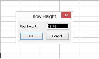
4. Enter the new row height and click on the OK button.
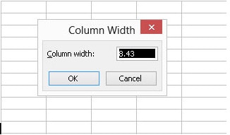
CHANGING COLUMN WIDTH:
The default column width in an Excel worksheet is 8.43 points. To change the column width for several columns at once, the steps are.
The default column width in an Excel worksheet is 8.43 points. To change the column width for several columns at once, the steps are.
- Select the column by dragging the mouse through the columns headings.
- Click on the Format menu.
- Choose the column option
- Then select the Width option from the drop down list.
- The column width dialog box is displayed.
- Enter the new column width in the Column width box and click on the OK button.
Using autofilL:
Excel Auto fill feature lets you enter predefined series of data such as text or numbers quickly.
For example:
January, February, ………….December
Sunday, Monday……………Saturday
1,2,3…………………………
1,3,5…………………………
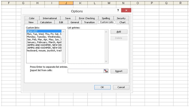
CREATING CUSTOM LIST:
Excel provides a feature that allows you to create your own custom list of names or text. After you have created a custom list you can use it to fill a range of cells.
The steps to create a custom lists are.
- Click on the tools menu.
- Select options
- Select the custom list tab.
- Select NEWLIST in the custom lists box
- Click in the list entries box and type each item that you want in your list.
- Click on the Add button to include the list in the Custom List box.
- Click on the OK button.
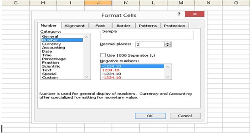
FORMATTING NUMBERS, DATE AND TIME:
Formatting changes the appearance of data, it does not affect its value. To format number, date and time,
you need to follow these steps-
Formatting changes the appearance of data, it does not affect its value. To format number, date and time,
you need to follow these steps-
- Select the range of cells whose data is to be formatted.
- Click on the Format menu and select the Cells options.
- The Format Cells dialog box is displayed. Select the number tab.
- Select the required category.
- Choose the desired format from the type option.
- Click on the OK button.
ERROR RESULTS:
Sometimes you get an error instead of a value as a result of a calculation. Here is a list of common error results that Excel returns.
##### The column is not wide enough to display the number. So must either widen the column or reduce the font size.
# DIV/0 ! Dividing by zero is an invalid operation.
# N/A Data is not available.
# Value ! The formula contains an invalid operator.
# Name ? A text string has not been enclosed in double quotes
# Null You included a space between two ranges in a formula to indicate an intersection.
# Num You supplied an invalid argument to a worksheet
# Ref You deleted a range of cells whose references are included in a formula.
Functions and Formula:
1- SUM( ): This function adds all the numbers in a range of cells.
2- MIN ( ): This function returns the smallest value of a set of values.
3- MAX ( ): This function returns the largest value of a set of value
s.
4- AVERAGE ( ): This function returns the average of the arguments.
5- CONCATENATE ( ): Joins several text strings into one text string.
6- EXACT ( ): Checks whether two text strings are exactly the same and returns TRUE or FALSE.
Exact is case sensitive.
7- FACT ( ): Returns the factorial of a number.
8- RIGHT ( ): Returns the specified number of characters from the right side of a string.
9- LEFT ( ): Returns the specified number of characters from the left side of a string.
10- LOWER ( ): This function returns the text in lower case.
11- UPPER ( ): This function returns the text in upper case.
12- SQRT ( ): This function is returns the square root of the number.
13- POWER ( ): This function is returns the power of the number.
Min =min(first value:last value)enter
Max =max(first value:last value)enter
Count =count(first value:last value)enter
Average =average(first value:last value)enter
Fact =fact(number) enter
Multiply =(first value*second value)
Div =(first value/last value)
Sub =(first value- last value)
Percentage =(first value*100/second value)
Sqrt =sqrt(number)
Power =power(number, power number)
Current date and time =now()
Current date =today()
Upper =upper(text)
Lower =Lower(text)
Mod =Mod(number, second number)
Discount =first price *(1-discount price)
Tax =first price* (1+tax price)
Concatenate =concatenate(first value, second value, third value)
Grade =if(h2>=90, "A", if(h2>=80, "B", if(h2>=70, "C", if(h2>=60, "D","F"))))
AUTOSUM FEATURE:
One of the most frequently used functions is the SUM ( ) that calculates the total of a set of numeric values. A toolbar button has been provided to invoke the SUM ( ) function. The AUTOSUM button will total the values above the destination cell.
SORTING DATA:
Sort means to arrange the given data according to a particular field, either in ascending or descending order. To sort the data follow the steps –
Sometimes you get an error instead of a value as a result of a calculation. Here is a list of common error results that Excel returns.
##### The column is not wide enough to display the number. So must either widen the column or reduce the font size.
# DIV/0 ! Dividing by zero is an invalid operation.
# N/A Data is not available.
# Value ! The formula contains an invalid operator.
# Name ? A text string has not been enclosed in double quotes
# Null You included a space between two ranges in a formula to indicate an intersection.
# Num You supplied an invalid argument to a worksheet
# Ref You deleted a range of cells whose references are included in a formula.
Functions and Formula:
1- SUM( ): This function adds all the numbers in a range of cells.
2- MIN ( ): This function returns the smallest value of a set of values.
3- MAX ( ): This function returns the largest value of a set of value
s.
4- AVERAGE ( ): This function returns the average of the arguments.
5- CONCATENATE ( ): Joins several text strings into one text string.
6- EXACT ( ): Checks whether two text strings are exactly the same and returns TRUE or FALSE.
Exact is case sensitive.
7- FACT ( ): Returns the factorial of a number.
8- RIGHT ( ): Returns the specified number of characters from the right side of a string.
9- LEFT ( ): Returns the specified number of characters from the left side of a string.
10- LOWER ( ): This function returns the text in lower case.
11- UPPER ( ): This function returns the text in upper case.
12- SQRT ( ): This function is returns the square root of the number.
13- POWER ( ): This function is returns the power of the number.
- =NOW( ) Current Date and Time
- =TODAY ( ) Current date
- =MOD ( ) Show the number of reminder
Min =min(first value:last value)enter
Max =max(first value:last value)enter
Count =count(first value:last value)enter
Average =average(first value:last value)enter
Fact =fact(number) enter
Multiply =(first value*second value)
Div =(first value/last value)
Sub =(first value- last value)
Percentage =(first value*100/second value)
Sqrt =sqrt(number)
Power =power(number, power number)
Current date and time =now()
Current date =today()
Upper =upper(text)
Lower =Lower(text)
Mod =Mod(number, second number)
Discount =first price *(1-discount price)
Tax =first price* (1+tax price)
Concatenate =concatenate(first value, second value, third value)
Grade =if(h2>=90, "A", if(h2>=80, "B", if(h2>=70, "C", if(h2>=60, "D","F"))))
AUTOSUM FEATURE:
One of the most frequently used functions is the SUM ( ) that calculates the total of a set of numeric values. A toolbar button has been provided to invoke the SUM ( ) function. The AUTOSUM button will total the values above the destination cell.
SORTING DATA:
Sort means to arrange the given data according to a particular field, either in ascending or descending order. To sort the data follow the steps –
- Select the cell in the worksheet.
- Select the Data menu and from the drop down menu select Sort option.
- The Sort dialog box is appear.
FILTERING DATA:
The filter command allows you to view only those records that meet certain specified rules. You can filter data using Auto filter.
USING THE Auto Filter:
There are various types of charts in MS- Excel. Make the charts on your worksheet.
The filter command allows you to view only those records that meet certain specified rules. You can filter data using Auto filter.
USING THE Auto Filter:
- Click on any cell in a worksheet carrying data.
- Click on the Data menu.
- From the drop down menu, Select Filter and then select Auto filter.
- Drop-Down controls will be display next to each field.
- You can click on any of the drop down controls to apply a filter to that particular fie
- Select the cells option from the format menu.
- Format cells dialog box is displayed.
- Click the Alignment tab.
- Choose Wrap text.
There are various types of charts in MS- Excel. Make the charts on your worksheet.
- Select the range of your data.
- Click the Chart button on the Standard toolbar or Click the Insert menu.
- Choose the Chart option.
- The Chart Wizard is displayed on your screen.
- Select the Chart type than click the next button.
- Select data range click the next button.
- Type the Chart title than click the next button.
- Click the finish button.
- Select the row or column.
- Click the Window menu and choose the Freeze Panes option.
